Understanding the Original Daisyworld Model

In the first attempt at the Metropolis Daisyworld Model, I didn’t do a great job of modeling the radiation from the sun and handling the latitude of the world. This led an incomplete model and so in this page, we are going to work through some corrections to this model. Here we go.

Understand How to Solve

Now I went back to building the first daisyworld model that was published in 1983 by Watson and Lovelock. It involved solving two coupled first order differential equations. Wow! That is a mouthful but not so hard when you think about. Consider the general case:

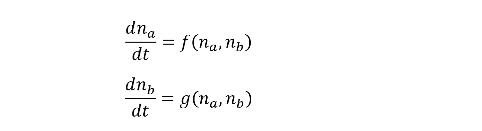
Where f and gare some complicated mathematical functions which we can use the computer to calculate. t is time. n_b is the percent of the population in state a (think BlackDaisies) and n_a is the percent of the population in state b (think WhiteDaisies).

Getting started on solving this, we can just cross multiply.

And of course n_a and n_b refer to the change in the populations (final – initial).

[Discussion question 1] what is the difference between dt and (delta)t? You may not know, that is fine. Find a friend who as taken calculus and have them explain it to you. Its pretty simple yet its implications are so powerful and complex it used all the time in mathematics.

Quickly solving these equations we get:

What is great about these equations is that as long as you know what the state is at some initial time (that is the 0) you can calculate the state of things at some final time that is given by t + dt. Weird right? This is called the Euler method. It has some issues, which we will not discuss. But it is a great starting point or solving this system.

So now we can daisy chain (HA HA HA) and bunch of these equations together to find the approximate value of n_a and n_b at all times. See on the graph how you extend the equation to:

So as long as you know what the value it at some time i, you can find the values at i+1. Well how do you know what the values are at i, you have to look back to i-1. You can keep looking back too. All the until you get to an initial state:

[Discussion Questions 2] What would the equations be for n_a2 and n_b2?

Now we have a way to calculate some stuff. Let’s do a quick example.

# Euler method
import matplotlib.pyplot as plt
import numpy as np

na    = 1
nb    = 0

dt    = 1
t     = 0

steps = 10

plt.plot(t,na,'bo')
plt.plot(t,nb,'ro')

for ii in range(steps):
    ff    = na + nb  #This is f and it depends on whatever you want it to
    gg    = -na + 2 * nb  #This is g.  f and g can be set to anything.  
    #Depend on the science
    
    #now do Euler
    na    = na + ff * dt
    nb    = nb + gg * dt
    t     = t + dt         #It is important to update your clock too.
    
    plt.plot(t,na,'bo')
    plt.plot(t,nb,'ro')

[discussion question 3] Run the code. Try changing ff = 4 and gg = n_b. What kind of plot do you get? Please explain your results. Try something else and then explain what you see.

Euler method to daisy model

The equations that are put forth in the daisy model are shown here:

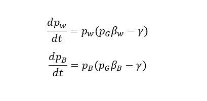
p_w – Population of white daisies
p_b – Population of black daisies
p_G – Population of ground without daisies (1 = p_w + p_b + p_G), they all add to 100%
gamma – dealth rate
beta_w and beta_b are complicated. These are the factors that tell you how the daisy will grow. I will discuss below.

Determining Beta

beta is a probability function. The orginal paper makes a guess on what it should look like. They said it should have the for:

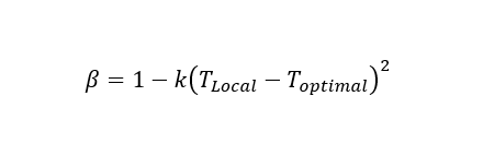
But only when beta is positive. Otherwise it is zero. k is a constant, T_Local is the temperature at the site in the world and T_Optimal is the optimal temperature for daisies to grow. There is an equation for both the white daisies and the black daises.

[discussion question 4] What are the situtations when the above equation is zero?

To determine the temperature of the Earth, we use the Stefan–Boltzmann law.

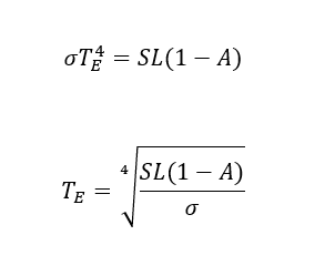
Where SL is the energy from the sun
A is the albeto of the earth
Sigma is the Stefan–Boltzmann constant

This is an equation you can look up in a physics textbook for how energy depends on temperature.

Calculating the Albeto of the earth is a little tricky. We do this by A = popW * aw + popB * ab + ag * popG, where aw, ab, and ag are the albetos of white daisies, black daisies, and the ground. When then approximate a change to the local temperature, given by:

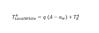
Putting everything together, we get the following code:

import numpy as np
import matplotlib.pyplot as plt

NumberSteps = 100
SL0         = 917   #solar output factor
sig         = 5.67e-8   #Stefan-Boltzmann constant
q           = 2.1e9     # q factor in model

aw          = 0.75  #albeto for white daisy
ab          = 0.25  #albeto for black daisy
ag          = 0.50  #albeto for ground

Topt        = 295.5 #optimal Temp
k           = 1/(17.5)**2  # K - parameter
gamma       = 0.1   #death rate
p           = 1     # factor of world that is avaliable for daisy

popW        = 0.3     # population of white
popB        = 0.3    # population of black

tt          = np.arange(0,NumberSteps,1)
SL          = SL0 * (1 + 0.0 * np.cos(tt/20))
POPW        = np.zeros(NumberSteps)
POPB        = np.zeros(NumberSteps)
TT          = np.zeros(NumberSteps)


for ii in range(NumberSteps):
    
    popG    = p - popW - popB
    #Find the albeto
      
    A       = popW * aw + popB * ab + ag * popG
  
    #EarthTemperature  note power to the fourth
    TEarth  = (SL[ii] * (1-A)  / sig)**0.25
    TT[ii]  = TEarth

    #determine local Temperautre
    TLocW   = (q * (A-aw) + TEarth**4)**0.25
    TLocB   = (q * (A-ab) + TEarth**4)**0.25
    TLocG   = (q * (A-ag) + TEarth**4)**0.25

    
    #Evaluate beta
    if (TLocW - Topt)**2 > 1/k:
        betaW = 0
    else:
        betaW = 1 - k * (TLocW - Topt)**2        
        
    #Evaluate beta
    if (TLocB - Topt)**2 > 1/k:
        betaB = 0
    else:
        betaB = 1 - k * (TLocB - Topt)**2                
        
    #use Euler to solve
    popW      = popW + popW * (popG * betaW - gamma)
    popB      = popB + popB * (popG * betaB - gamma)
    
    
    POPW[ii]   = popW
    POPB[ii]   = popB
    
plt.subplot(211)
plt.plot(tt, POPW, '-r')
plt.plot(tt, POPB, '-b')
plt.xlabel('Times')
plt.ylabel('Population')

plt.subplot(212)
plt.plot(tt, TT, '-r')
plt.xlabel('Times')
plt.ylabel('Temp (K)')

[discussion question 5] Run the code and identify which lines of code coorspond to which equations?

In Line 22, we adjust the radition of the sun.

SL          = SL0 * (1 + 0.1 * np.cos(tt/20))

Play with this equation and run it.

Check it out with 20% fluctuations in solar radiation, this is what the daisies do? The Earth’s temeprature barely moves (10/300) ~ 3% fluctuations.

Pretty neat.

My next steps would be to play with the solar radiation to see what will happen.

[discussion question 6] Was it helpful to try the “First Attempt At Metropolis Daisyworld Model” before do the original model?

Understanding the Original Daisyworld Model

Like this: